When does distillation help reinforcement learning?

Introduction

We are very interested in the interplay between distillation and reinforcement learning. Evidently, much of the advancement in capabilities in LLMs as of late has been due to scaling up RL, both in compute and number of environments. Distillation is often seen as a way to warm-start a model in preparation for RL. This is because in RL we need a non-zero starting reward with a model in order to be able to hill-climb, and if we can go from zero to non-zero by training on a few traces from a better model, then we unlock the value of the whole RL environment.

Distillation is thus seen as a crutch used by open-source model labs as a way to stay within a stone’s throw of the closed-source labs with stronger models. However, it is unclear about how distilling from a stronger model can affect the ceiling (and floor) with respect to the capabilities of the model you are training. Here lie some interesting questions:

How much does being on-policy in distillation matter? For instance, if I am training on a completely different model family, will this later fry my model? Will it somehow decrease the entropy? How much RL do I need to repair this?
Suppose I have a fixed compute budget. What is the optimal dose of distillation vs RL? Assuming more distillation is not always monotonically better, this can give us an interesting result.

Based on the core idea behind these questions, we study whether SFT on teacher-generated solutions improves subsequent RL. We compare Qwen3 models with 0.6B, 1.7B, 4B, and 8B parameters, trained with GRPO either directly or after fine-tuning on verified teacher solutions, across sixteen reasoning tasks. We find that distillation helped improve accuracy before RL at every model size, but its benefit after RL depended both on the student size (e.g. Qwen3) and task. Smaller models (0.6B and 1.7B) retained substantial gains that increasingly diminished at larger sizes (4B and 8B). Indeed, at 8B, the model trained with RL alone performed better overall, although this improvement was concentrated in a subset of calculation tasks. Together, our results show that higher accuracy prior to RL (due to distillation) does not necessarily yield higher accuracy after RL, with distillation becoming less valuable as the size of the student increases.

Experimental setup

We used Qwen3 models with 0.6B, 1.7B, 4B, and 8B parameters. At each size, we compared RL only, which applies GRPO directly to the base checkpoint, and SFT + RL, which first finetune the same checkpoint on teacher-generated solutions with SFT. Throughout this work, distillation refers to the supervised training on teacher responses.

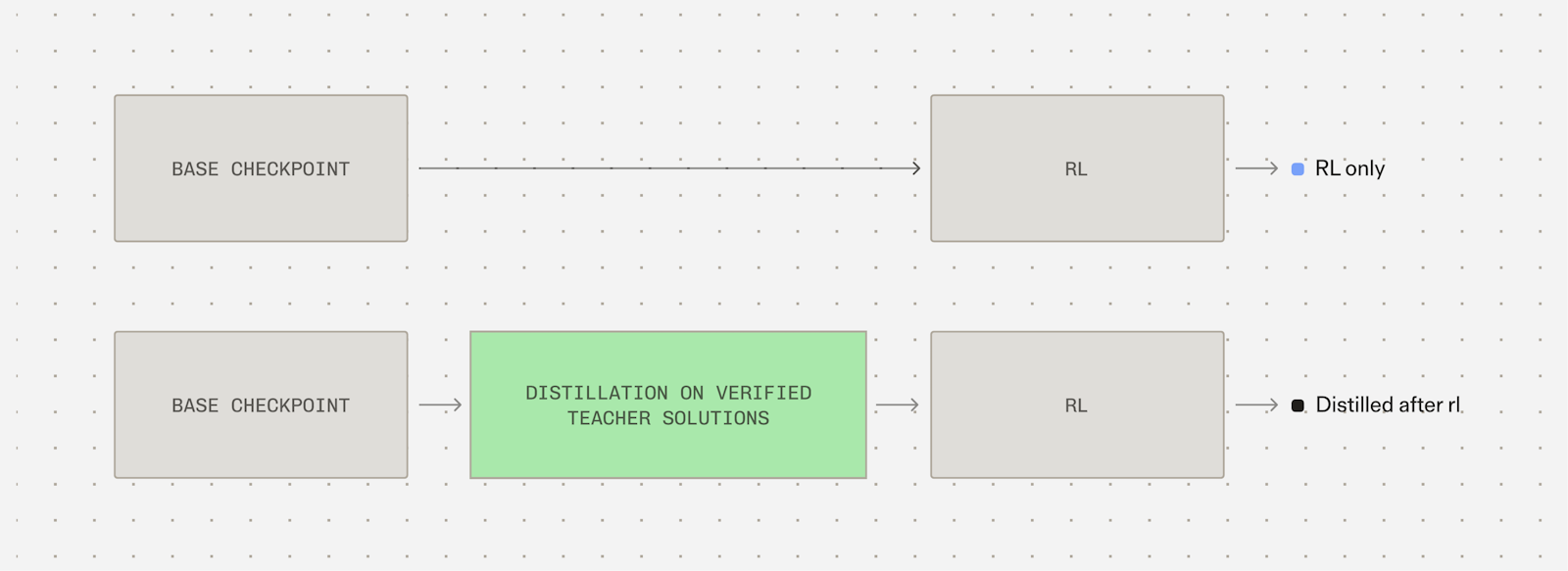
schematic — Figure 1
Both training conditions use the same base checkpoint, with RL-only applying RL directly whereas distillation (SFT + RL) first fine-tunes the checkpoint on verified teacher solutions, then applies RL.

To generate SFT data, we used a fixed teacher, gpt-5.6-sol. Each student was fine-tuned on subsets of data containing 0.5M, 1M, 2M, or 4M of these teacher-response tokens (these were constructed such that larger datasets contained the smaller subsets).

Our main experiment compared the RL baseline with SFT on 2M response tokens, followed by RL. We repeated RL training three times for each starting condition at each model size. To examine how the amount of SFT data affected performance, we also ran RL once for every combination of student and data size, including the RL baseline.

Teacher-generated training data

The student was trained in raw completion format. We did this to avoid the confound of distillation teaching a chat format. Each example concatenated a problem prompt with a teacher response. The prompt was masked out of the SFT loss and minimized the next-token cross-entropy on the teacher response and its appended end-of-sequence token. Here is an example (we include line breaks for readability):

Prompt — excluded from the SFT loss:

Solve each problem. Reason step by step if needed, then write
exactly one final answer between `<answer>` and `</answer>`
tags. The closing `</answer>` tag must be the final text you
write. Stop immediately after it and do not write anything else.

Problem:
Tell me whether 2116 is a leap year. Answer with Yes or No.

Solution:

Target — included in the SFT loss, including the appended EOS:

<think>2116 is divisible by 4 and not divisible by 100, so it is
a leap year under the Gregorian
rules.</think><answer>Yes</answer><|endoftext|>

Teacher responses contained a written derivation within <think> tags and a final answer within <answer> tags. We retained only correct responses completed without reaching the generation limit, and satisfied task-specific length (from 256 to 1,536 tokens) and formatting checks. Appendix A describes the preliminary experiments used to develop these procedures.

Tasks

We selected sixteen tasks from Reasoning Gym (Stojanovski et al., 2025), a library of generated reasoning problems with verifiable answers. For these problems, we generated training and evaluation instances at different difficulty levels and grouped the tasks into eight calculation tasks and eight structured tasks. For instance, calculation tasks included problems such as multiplication or fractions, Appendix B provides exact task details.

Results

Benefit of distillation depends on student size

Fine-tuning on 2M tokens improved accuracy before RL at all student sizes. The initial improvement was larger for smaller model sizes, increasing accuracy by 31.2% at 0.6B compared with 15.3% at 8B. We then looked at whether these improvements persisted after RL (Figure 2).

Here we found mixed results. After each model had generated 80 million response tokens during RL training, SFT+RL outperformed RL by 11.3% at 0.6B, 13.1% at 1.7B, and only 2.1% at 4B. When scaling up to 8B, RL outperformed SFT+RL by 6.4%. The benefit of distillation after RL therefore decreased with student size, with the changes from 0.6-8B amounting to a decline of 17.8% (bootstrap 95% CI: 6.7-31.0) and the fitted relationship between distillation benefit and log student size coming out negative in each of the three runs.

These results show that improving accuracy before RL does not necessarily improve accuracy after subsequent training, although we note that this conclusion applies to the training budget that we evaluated. Further, given that the size of the student model changes both model capacity and the pretrained starting policy, we are unable to establish capability differences between the teacher and student as the cause of this phenomenon.

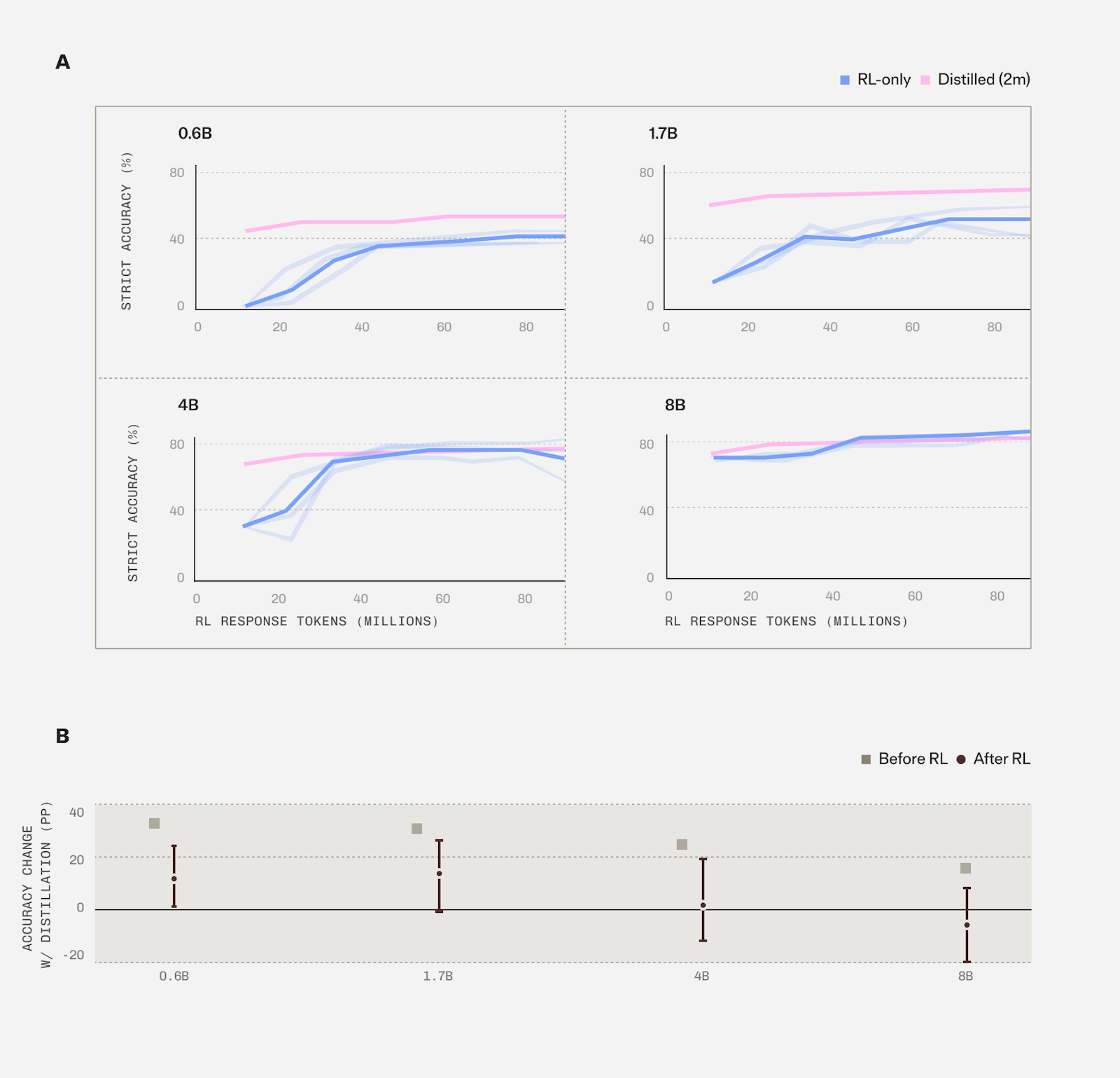
Figure 2
Effect of distillation across student sizes. (A) Strict accuracy during RL, plotted against generated RL response tokens. Faint lines are individual runs and darker lines are the mean. (B) Difference in strict accuracy between SFT + RL and RL-only before RL (squares) and after 80M RL response tokens (circles). Positive values favour SFT + RL.

Benefit of the amount of distillation

Up until this point, our comparisons have used distillation with 2M teacher-response tokens. We further varied this amount, from zero to 4M tokens, to examine whether more distillation provides a better starting point for RL.

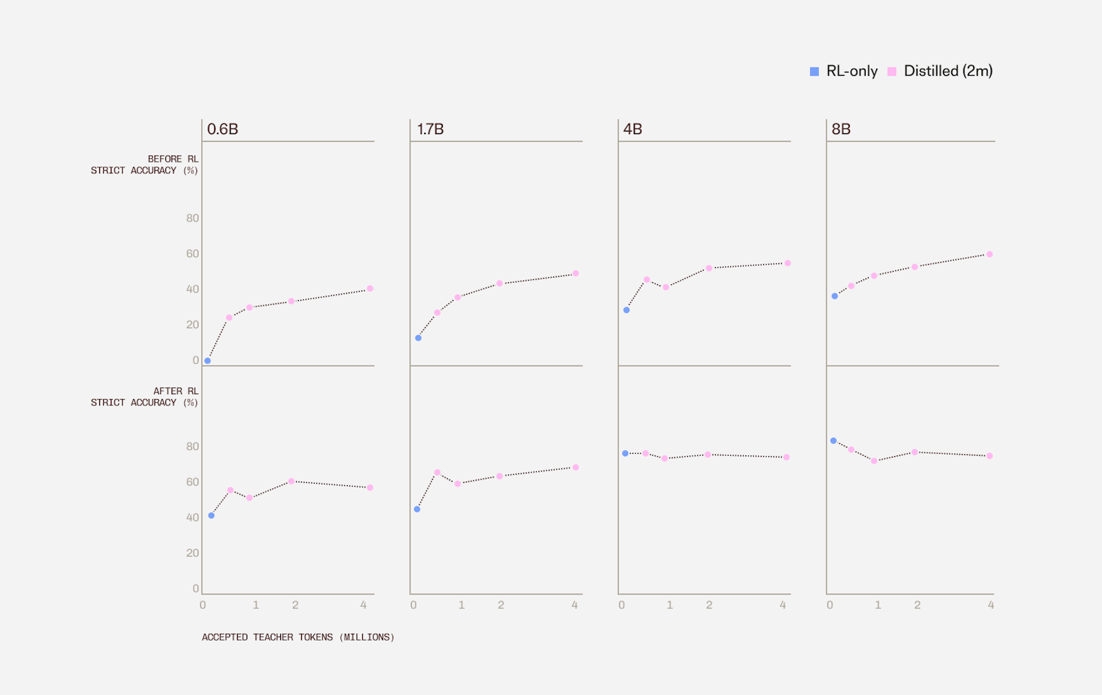
Figure 3
Strict accuracy by student size and amount of distillation data (0, 0.5M, 1M, 2M, or 4M tokens). Top row shows accuracy after SFT and before RL; bottom row shows accuracy after 80M RL response tokens. We show one RL run per condition.

Our results were inconsistent across the conditions we tested. For example, our best endpoint used 2M teacher tokens at 0.6B and 4M at 1.7B, as opposed to 4B which recorded best accuracy with zero and 0.5M tokens. Strengthening our earlier results, at 8B the base model (without distillation) outperformed every distilled starting point after RL. Thus, a greater amount of distillation tokens did not improve the model obtained after subsequent RL. This further suggests that it is tricky to select the target amount of distillation purely by measuring downstream accuracy after such SFT alone, without considering the subsequent accuracy after RL too.

The effect of distillation between task categories

We further dissected the performance of different training combinations on different tested tasks. For instance, base models matched or exceeded distilled models at every student size in calculation tasks, whereas in structured tasks distillation retained a notable advantage.

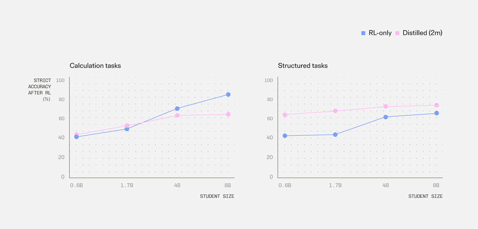
Strict accuracy after RL by student size for calculation and structured tasks, comparing RL-only and distilled (2M) models; both x-axes include 4B. — Figure 4
Scale trends for undistilled vs. distilled models, split by task type. While RL can overtake distillation gains for “calculation” tasks (e.g. polynomial equations, simple integrals), distillation maintains a strict advantage for “structured” tasks (e.g. reversing spelling). Further details of task split can be found in Appendix B

We further controlled for semantic-correctness and the tendency of models to learn the ‘right format’ not evident in strict accuracy measures (see Appendix G). Here we observed that at 4B and 8B, distilled models did indeed follow the required format answer more reliably.

One hypothesis for these findings is that in tasks that require specific convention or understanding, such as how to properly rotate a cube, particular demonstrations of this knowledge could be useful. Contrastingly, in more direct calculation, the larger pretrained model may discover some calculation procedure directly from reward.

Could differences in the starting policy explain these results?

We next examined whether differences between the starting models could help explain their subsequent performance. We considered two possibilities. First, that smaller base models initially generated too few correct responses to provide a useful GRPO training signal, and second, that SFT changed the model’s next-token entropy in a way associated with later accuracy.

How often did the starting models generate correct responses?

We examined 1.7B, 4B, and 8B models across all five SFT data amounts. Before RL, we sampled sixteen responses to each of 64 prompts for these models and measured how often the starting models generated correct answers.

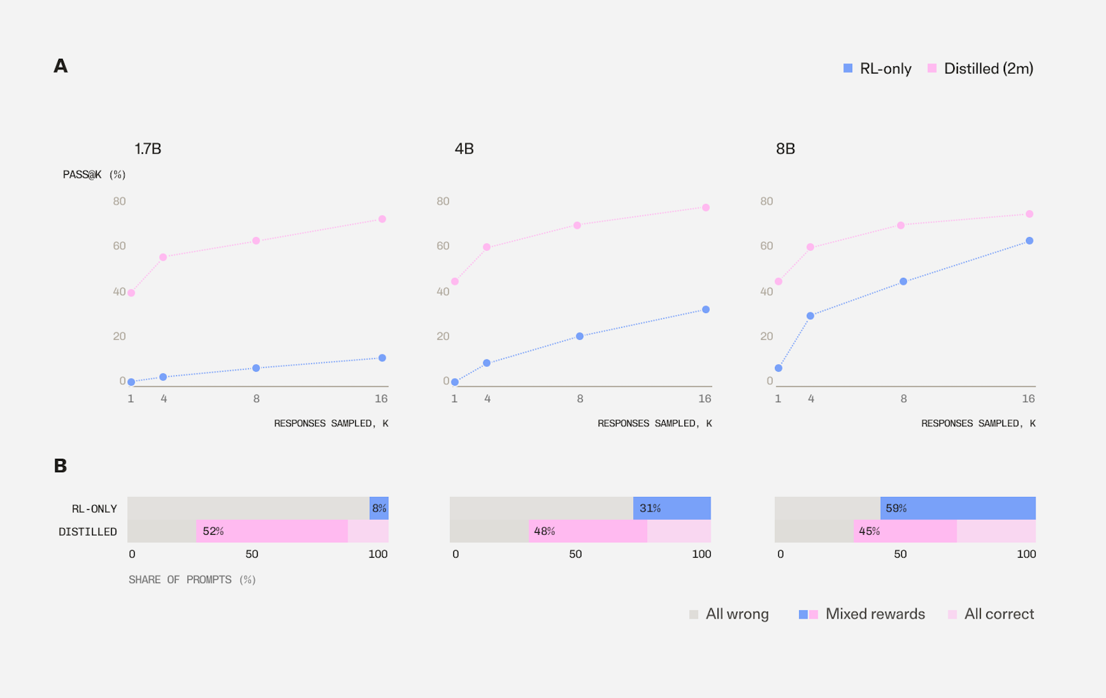
Figure 5
Further RL diagnostics for distilled vs. undistilled models at various scales. Pass@k curves ideally increase non-negligibly (A - top), and groups of responses ideally have a mix of correct and incorrect responses (B - bottom). As we scale, base models are healthier in terms of these two metrics, while distilling can both flatten pass@k curves and reduce the amount of mixed reward groups.

Before SFT, the base models generated at least one correct response in sixteen attempts for 7.8% of prompts at 1.7B, 31.2% at 4B, and 59.4% at 8B. After SFT on 2M teacher-response tokens, these proportions were 70.3%, 73.4%, and 68.8%, respectively. SFT therefore increased initial success most strongly for the 1.7B model, largely removing the differences between model sizes.

However, a useful GRPO training signal must contain responses with different rewards. That is, groups must contain both correct and incorrect responses to provide nonzero advantages. For a fixed prompt, let p denote the probability that a sampled response receives reward one. Assuming sixteen independent responses from the same policy,

\begin{aligned} P(\text{at least one correct})&=1-(1-p)^{16},\\ P(\text{mixed rewards})&=1-(1-p)^{16}-p^{16} \end{aligned}

Increasing p therefore increases the probability of finding at least one correct answer, but does not always increase the probability of obtaining mixed rewards. As correct responses become more likely, groups can also become entirely correct, leaving no relative reward signal.

We therefore measured the proportion of these mixed groups before RL. At 1.7B, SFT on 2M teacher-response tokens increased this proportion from 7.8% to 51.6%. At 4B, it increased from 31.2% to 48.4%. At 8B, however, it decreased from 59.4% to 45.3%, while the proportion of ‘100% correct’ groups increased from zero to 23.4%. Thus, our results show that SFT did not always increase the proportion of prompts providing a relative reward signal, and are consistent with SFT helping smaller models begin RL with more useful training responses.

Does distillation change next-token entropy?

We next examined whether distillation changed next-token entropy, and whether these differences persisted after RL. The intuition for this analysis is that entropy measures how concentrated the model’s next-token probabilities are, with lower entropy meaning that probability is concentrated on fewer tokens.

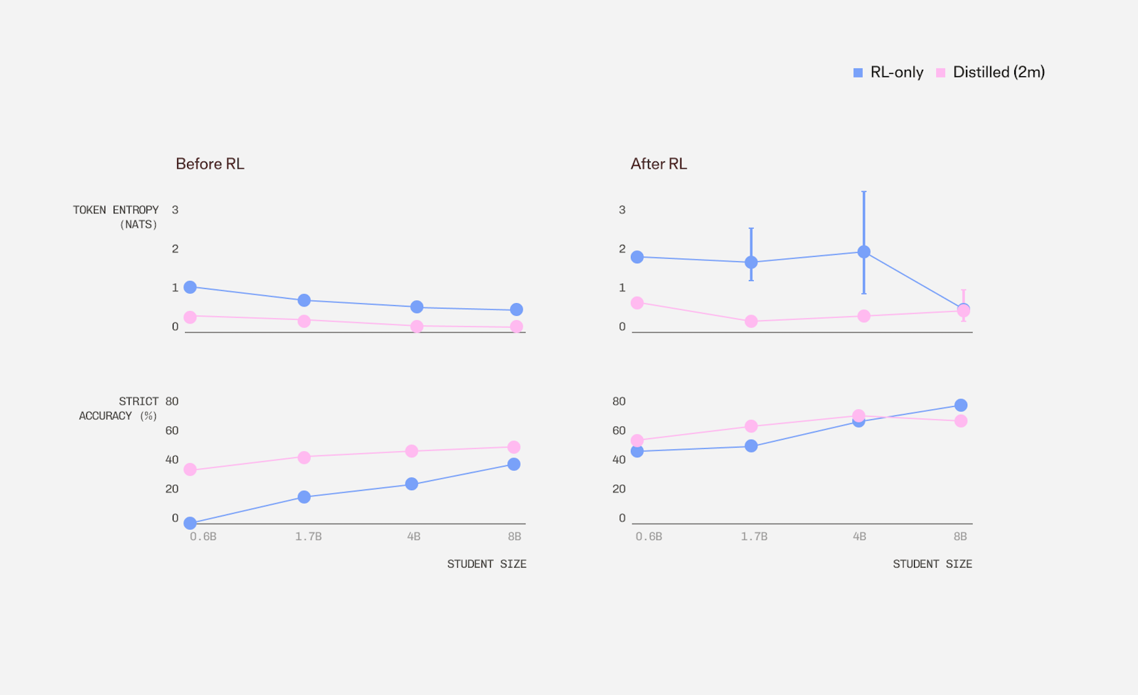
Figure 6
Next-token entropy on fixed reference solutions and the corresponding accuracy comparison, before and after RL. Distillation consistently reduces entropy throughout settings, with the exception of the performance crossing point where the distilled model is worse, where we see the non-distilled model’s entropy decrease substantially.

To do this, we evaluated every model on the same 64 reference solutions, with four solutions per task. At each position, we supplied the problem and the preceding reference tokens, then measured entropy over the model’s next-token distribution. This allowed us to compare models on identical inputs.

For a model with parameters $\theta$ , problem $x_i$ , and reference solution $y_i$ containing $L_i$ tokens, we calculated:

H(\theta)=-\frac{1}{\sum_i L_i}\sum_i\sum_{t=1}^{L_i}\sum_v \pi_\theta(v\mid x_i,y_{i,<t})\log\pi_\theta(v\mid x_i,y_{i,<t}).

We calculated entropy (in nats) over the full vocabulary using next-token probabilities, then averaged across all reference-response tokens (this includes the final end-of-sequence token but excludes the prompt).

We found that SFT reduced next-token entropy before RL across all student model sizes (Figure 6), which was accompanied by higher accuracy. In other words, given the same problem and partial solution, models that were distilled were therefore less uncertain about which token to generate next. These trends were similar after RL for models from 0.6-4B. Interestingly, 8B had similar average entropy (0.691 nats for RL only and 0.699 for SFT + RL), despite RL only achieving marginally higher accuracy. Taken together, these results show that distillation often reduces next-token entropy both before and after RL, although this measure alone cannot explain overall accuracy differences.

SFT on teacher-generated solutions can help a model begin RL by increasing how often it generates correct responses. Beren Millidge argues that this initial improvement can support further learning, while much of the subsequent capability improvement comes from RL itself. Given this, related work has also examined how much compute to spend on distillation. Busbridge and colleagues have sought to understand how allocating compute between teacher and student affects the resulting student model. Here, our experiments examined whether initial improvements obtained during distillation persist after subsequent RL.

Part of our study involves studying how the amount of distillation plateaus. A close comparison to this is the work of Aphale and Liu, who find that additional SFT can improve accuracy before RL while reducing performance after GRPO. In our experiments, we varied teacher-response data from zero to 4M tokens across four student sizes, finding that “optimal” amount of distillation differed between sizes and further suggesting that higher accuracy after SFT alone is insufficient for choosing how much distillation to use before RL.

Other studies have also examined whether distillation followed by RL can increase the range of problems a model can solve. Kim and colleagues find that distillation can improve accuracy without consistently increasing the range of problems solved across multiple attempts. We examine whether these initial accuracy gains translate into better performance after RL, finding that they do not always persist. QuestA uses partial teacher solutions as hints during RL, improving performance even when those hints are removed at evaluation. ProRL shows that a distilled model can learn to solve additional problems through prolonged RL with measures to stabilise training. These results suggest that the benefit of teacher solutions largely depends on how subsequent RL is performed, indicating that our initial pass@k measurements are not a limit on how the model will later learn.

Finally, “distillation” covers different algorithms. Our experiments use SFT on fixed teacher-generated solutions, but other methods train on responses generated by the student model. Generalized Knowledge Distillation uses the teacher’s next-token probabilities to guide learning on these responses. Separately, RL’s Razor finds that RL can preserve previously learned capabilities better than SFT at similar accuracy on a new task. A future question we’re interested in is whether more on-policy or stronger forms of distillation can improve subsequent RL.

Summary

We showed that distillation improves accuracy before RL at every student size, but that these gains do not consistently persist through training after RL. Indeed, after 80M RL tokens, smaller students such as 0.6B and 1.7B retained the benefit of distillation, whilst this advantage diminished for 4B and reversed at 8B. We also found that the benefit of distillation depends on the trained task, with structured reasoning tasks benefiting from distillation, whilst calculation tasks largely depend on student size. Critically, across these findings, the amount of distillation did not consistently improve final accuracy.

Our results suggest that distillation is no “silver bullet” within the post-training regime. How (and how much) distillation is utilised depends on the student model, the tasks cared about and the RL budget. We provide no mechanistic reason for these observations, but suggest that understanding how different distillation or RL methods change these relationships remain important next steps.

Acknowledgments

We thank Dwarkesh Patel for his insights and discussions that motivated the completion of this work.

References

Agarwal, R., Vieillard, N., Zhou, Y., Stanczyk, P., Ramos, S., et al. (2024). On-policy distillation of language models: Learning from self-generated mistakes. ICLR 2024. arXiv:2306.13649
Aphale, S., & Liu, K. (2026). SFT overtraining predicts rank inversion via entropy collapse under RLVR. arXiv:2606.18487
Busbridge, D., Shidani, A., Weers, F., Ramapuram, J., Littwin, E., & Webb, R. (2025). Distillation scaling laws. ICML 2025, PMLR 267. proceedings.mlr.press/v267/busbridge25a
Kim, M., Shrestha, A., Shrestha, S., Nepal, A., & Ross, K. (2025). Reinforcement learning vs. distillation: Understanding accuracy and capability in LLM reasoning. arXiv:2505.14216
Li, J., Lin, H., Lu, H., Wen, K., Yang, Z., et al. (2025). QuestA: Expanding reasoning capacity in LLMs via question augmentation. arXiv:2507.13266
Liu, M., Diao, S., Lu, X., Hu, J., Dong, X., et al. (2025). ProRL: Prolonged reinforcement learning expands reasoning boundaries in large language models. arXiv:2505.24864
Millidge, B. (2026, June 12). Distillation ain't what it used to be. beren.io
Shao, Z., Wang, P., Zhu, Q., Xu, R., Song, J., et al. (2024). DeepSeekMath: Pushing the limits of mathematical reasoning in open language models. arXiv:2402.03300
Shenfeld, I., Pari, J., & Agrawal, P. (2025). RL's Razor: Why online reinforcement learning forgets less. arXiv:2509.04259
Stojanovski, Z., Stanley, O., Sharratt, J., Jones, R., Adefioye, A., et al. (2025). Reasoning Gym: Reasoning environments for reinforcement learning with verifiable rewards. arXiv:2505.24760

Technical appendix

A) Preparing teacher-generated training data

We tried many different approaches to generate the reasoning traces from the teacher, largely looking at multiplication. Our aim was to come up with a stable recipe for generating teacher traces that all students could learn from. One key decision was how concise or verbose to make the teacher outputs.

Brief solutions. Here is an example of a concise teacher where the question was 649 × 427. This accepted response contained 34 student target tokens:

<think>
649 × 427 = 277123
</think>
<answer>277123</answer>

Across the rollouts we accepted for the precise teacher, the median target length was 97 tokens and the 95th percentile was 304. Perhaps not surprisingly, the observed accuracy improvement after training the student on these teacher traces was limited. Obviously, just having a correct final number accompanied by little worked computation was not enough to imbue improvement.

Longer solutions. We also tested responses generated by Qwen3-32B. An accepted response to 8 × 7 × 2 × 8 × 4 × 5 × 8 contained 1,214 target tokens. This is an excerpt of its opening:

Okay, let's see. I need to multiply these numbers together: 8,
7, 2, 8, 4, 5, and 8. Hmm, that's seven numbers multiplied in a
row. Let me start step by step. Maybe I can group some numbers
to make it easier.

First, let me write them all out: 8 × 7 × 2 × 8 × 4 × 5 × 8. Let
me see if there are any pairs that multiply to something easier.
For example, 8 and 5. Wait, 8 × 5 is 40. That's a nice number.
Let me note that. Then maybe 4 × 5... oh wait, there's already a
5. Wait, the numbers are 8, 7, 2, 8, 4, 5, 8. Let me check
again.

The response continues through several ways of grouping the multiplication and returns the correct answer, 143360. We found that students trained using this procedure frequently reached the generation limit.

Step-by-step solutions. We then prompted GPT-5.6 to show the calculation step by step, without restarting or trying alternative approaches, and to use the result as its final answer. For 808 x 900, it produced:

<think>Since 900 = 9 × 100, compute 808 × 9 = 7,272, then
multiply by 100: 7,272 × 100 = 727,200. The exact product is
727,200.</think><answer>727200</answer><|endoftext|>

For multiplication, we required a correct final answer and checked intermediate arithmetic where possible. Accepted responses had a median length of 398 tokens and a 95th percentile of 936 tokens, under a 1,536-token limit.

B) Task selection and difficulty

Our initial experiments used four tasks consisting of multiplication, polynomial equations, cube rotation, and bit counting. We screened 24 candidate tasks using the training sampling settings, with 128 prompts per task and sixteen responses per prompt.

We sought tasks on which the starting/base model sometimes succeeded but still produced incorrect responses, giving GRPO variation in rewards within a prompt. Our initial selection criteria were pass@1 between 5% and 45%, pass@16 between 50% and 98%, a mean $p (1-p)$ of at least 0.03 (see above for rationale/formula), and fewer than 5% of responses reaching the generation limit.

This screening guided our choice of eight calculation and eight structured tasks, including the four used initially. We replaced candidates with problematic response lengths or answer checking. The table below lists the standard level of task difficulty used in the main experiments, and how each task changes in difficulty in the experiments described in Appendix F.

Group	Task	Main difficulty	Harder difficulty
Calculation	Calendar arithmetic	2	2 (unchanged)
Calculation	Decimal-chain sum	3	3 (unchanged)
Calculation	Fraction simplification	1	2
Calculation	Leg counting	13	16
Calculation	Polynomial equations	2	2 (unchanged)
Calculation	Products	5	7
Calculation	Simple integration	0	2
Calculation	Time intervals	3	3 (unchanged)
Structured	Cube rotation	1	3
Structured	Bit counting	1	2
Structured	Course scheduling	0	2
Structured	Anagram grouping	0	1
Structured	Star paths	0	1
Structured	Abstract grids (re-ARC)	0	1
Structured	Reverse spelling	1	2
Structured	Mini Sudoku	0	1

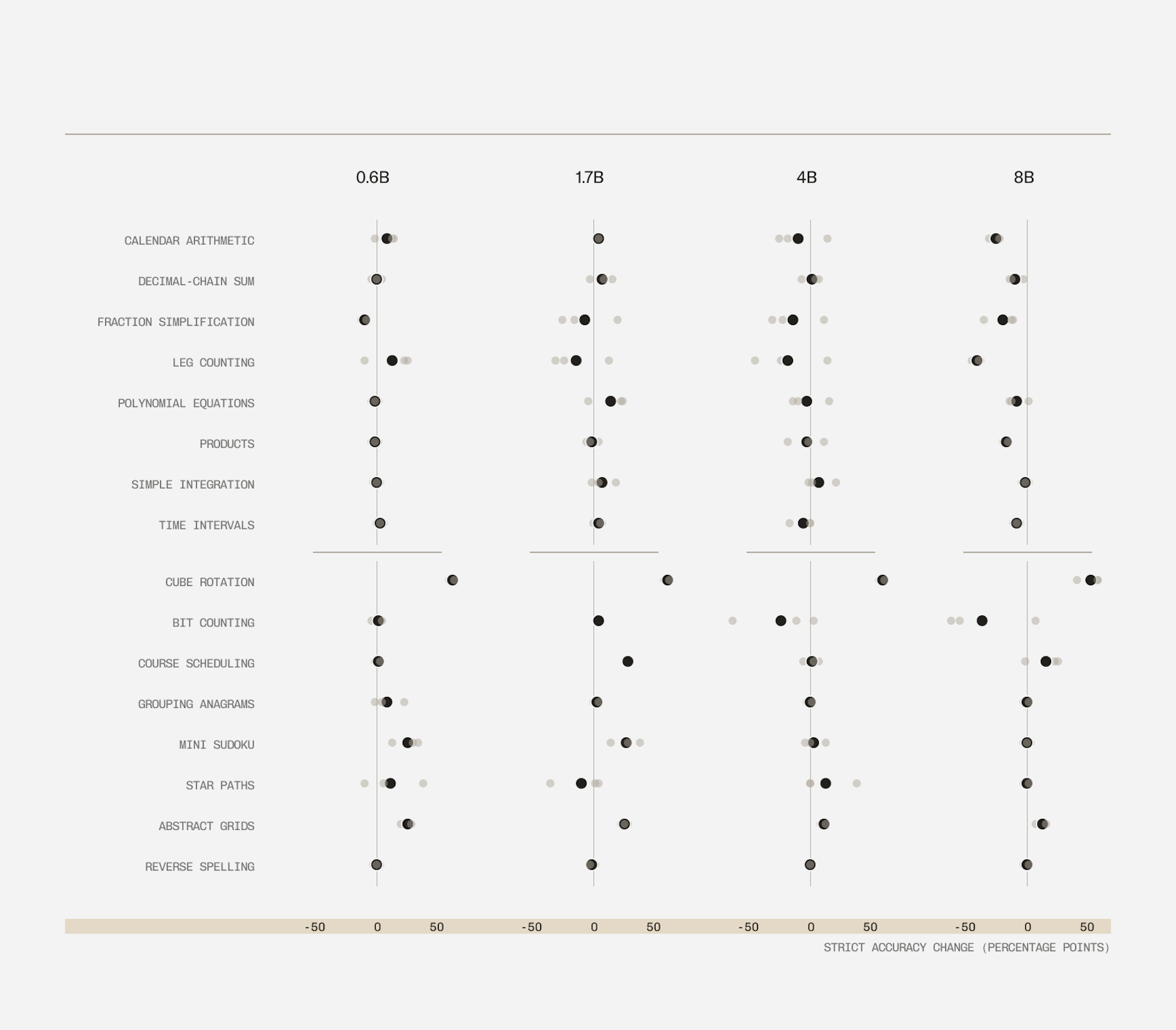
figurea1 — Figure 7
Individual task performance differences between distilled and undistilled models after RL. Faint points are paired training runs; dark points are mean.

C) RL objective and sampling settings

We used a GRPO-family objective with rewards normalised within each prompt’s group of responses. For prompt $i$ and response $j$ , the reward $r_{ij}$ was 1 if the response contained the correct answer in the required format and 0 otherwise.

Each group contained $G=16$ responses. We calculated the mean reward, standard deviation and normalized advantage as:

\begin{aligned} \bar r_i&=\frac1G\sum_j r_{ij},\\ s_i&=\sqrt{\frac1{G-1}\sum_j(r_{ij}-\bar r_i)^2},\\ A_{ij}&=\frac{r_{ij}-\bar r_i}{s_i+10^{-6}}. \end{aligned}

The same advantage was applied to every token in a response. Let $\rho_{ijt}$ denote the ratio of the updated policy’s probability to the probability under the policy used to generate token $t$ in response $j$ . With a clipping parameter of 0.2, the ordinary contribution was:

q(\rho,A)=\min\bigl(\rho A,\operatorname{clip}(\rho,0.8,1.2)A\bigr).

We also used a dual-clip bound of 3 for negative advantages:

\widetilde q(\rho,A)=\begin{cases}q(\rho,A),&A\ge0,\\\max(q(\rho,A),3A),&A<0.\end{cases}

And the training loss was:

\mathcal L=-\frac{\sum_{i,j,t}m_{ijt}\widetilde q(\rho_{ijt},A_{ij})}{\sum_{i,j,t}m_{ijt}}.

Here $m_{ijt}$ selects response-token positions, meaning that the loss is averaged over response tokens across the batch. Each batch of generated responses received one PPO epoch using a single minibatch containing all prompts (the recorded clipped fraction was 0).

We trained all parameters using AdamW with constant learning rate 3 × 10⁻⁶, betas (0.9, 0.999), weight decay 0.01, and gradient-norm clipping at 1.0. The policy model used bfloat16 and both KL coefficients and entropy coefficient were zero.

Our implementation follows the group-relative approach introduced in DeepSeekMath, with group-standardised advantages and token-level probability ratios.

Setting	Standard task RL	Hard task RL	Evaluation
Temperature	1.0	0.6	0.6
Top-p	0.95	0.95	0.95
Top-k	Disabled	20	20
Maximum response tokens	12,288	12,288	4,096
Responses per prompt	16	16	4

D) Comparisons at equal numbers of RL updates

Models initialised with SFT generally generated shorter responses, allowing them to complete more updates within the same RL budget. We therefore also compared models after equal numbers of updates.

Each update contained 1,024 rollouts. By matching update counts, we therefore also matched the number of responses generated during training – we estimated accuracy at 80, 96, and 112 updates. At 96 updates, SFT + RL exceeded RL only by 12.62 percentage points at 0.6B and 12.57 points at 1.7B. These changed reversed at larger model sizes, where differences were −5.69 points at 4B and −7.48 points at 8B, favouring RL only. These results were largely maintained at 80 and 112 updates.

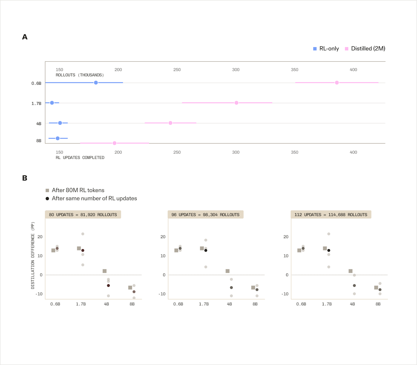
figurea2 — Figure 8
Comparison at equal numbers of RL updates. (A) Updates and rollouts completed by each condition; points show means and horizontal bars range. (B) Strict accuracy difference, SFT + RL minus RL-only, at 80, 96, and 112 matched updates (dark points), or the 80M token comparison (squares). Faint points are individual runs. Each update contains 1,024 rollouts.

E) Could distillation reduce the amount of RL needed to reach a target accuracy?

Much of our work has centred on final comparisons between RL and SFT+RL. It may be that some teams/companies rather want a model that reaches an acceptable accuracy quickly, instead of simply the highest accuracy at the end of a long run. We therefore measured when different token amounts first reached a specified accuracy during evaluation.

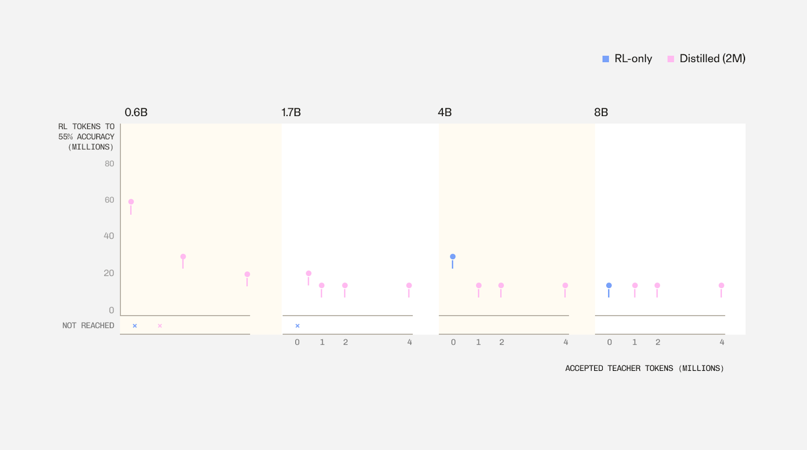
figurea3 — Figure 9
RL response tokens needed to first observe 55% accuracy, by student size and SFT data amount (one run per condition). Crosses indicate the target accuracy was never reached.

At a target accuracy of 55%, SFT reduced the amount of RL required at 4B, but did not produce an earlier observed crossing at 8B. Further, for lower student sizes, some models had already met the required accuracy after SFT, before any RL. We repeated this comparison at targets of 45%, 50%, and 60%, which also changed which training condition performed best.

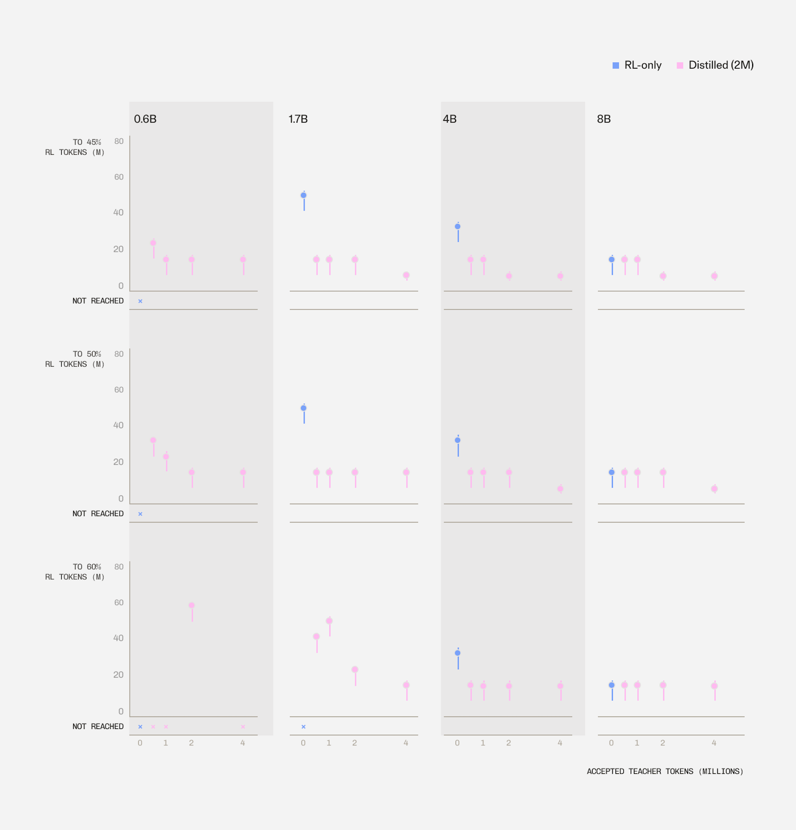
figurea4 — Figure 10
Analysis in Figure 9 repeated for 45%, 50%, and 60% strict-accuracy targets (rows). Dots mark the first evaluated checkpoint at or above a target; stems are the last checkpoint below and the first checkpoint above. Crosses indicate the target accuracy was never reached.

F) Training and evaluation on harder problems

We compared RL only and SFT + RL under standard and harder training and evaluation settings (Figure 11). The harder settings increased the difficulty of twelve tasks and left four unchanged (Appendix B). Distillation retained an advantage at smaller student sizes across both training settings.

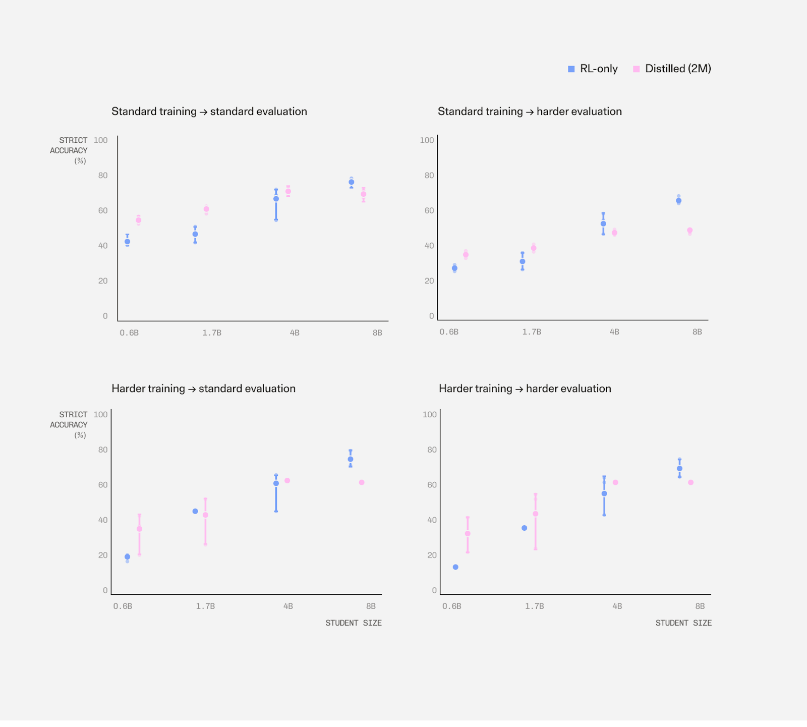
figurea5 — Figure 11
Strict accuracy across standard and harder training and evaluation settings, by student size. Points give means across three runs; bars give range.

G) Answer correctness and formatting

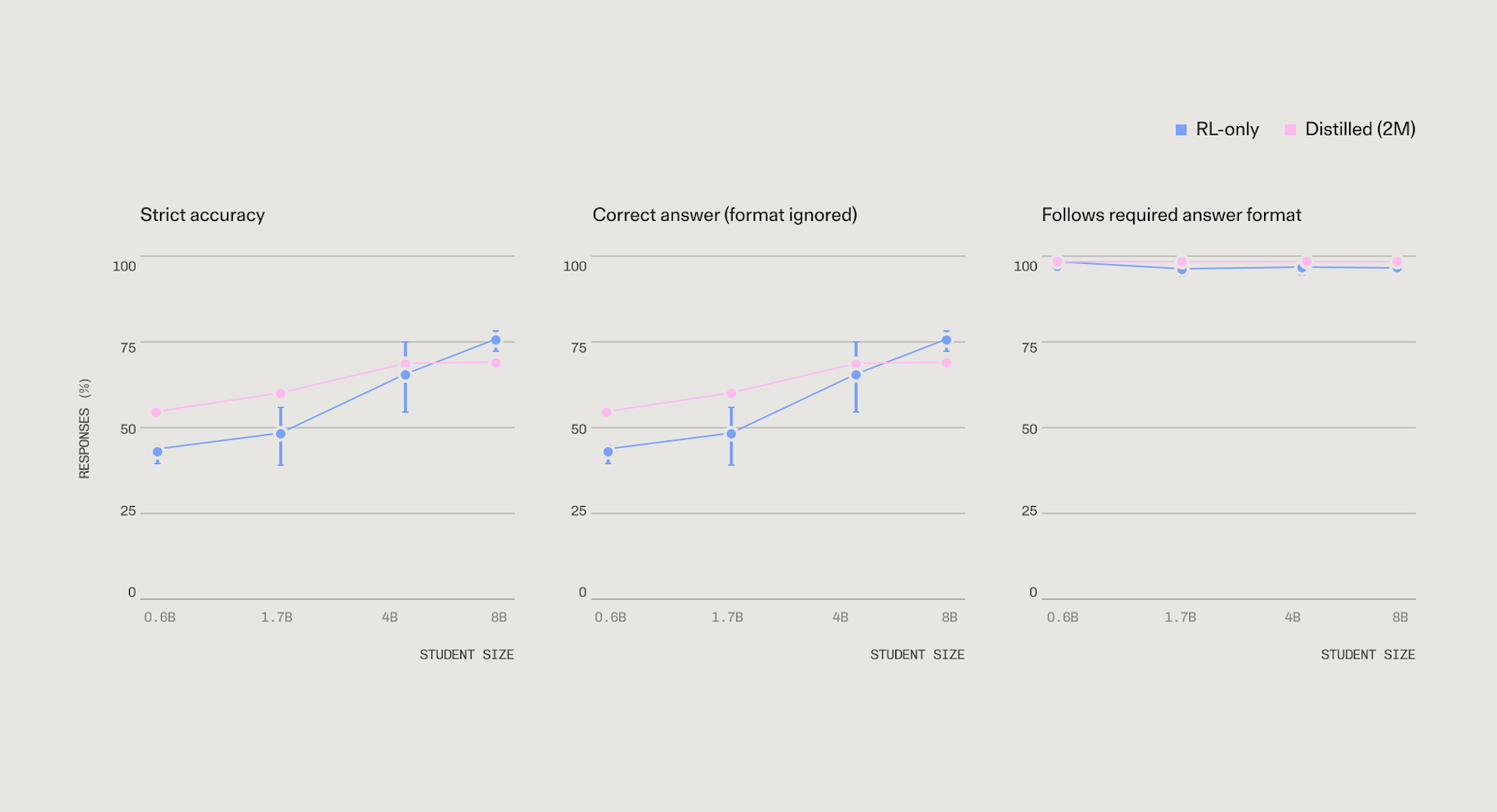
figurea6 — Figure 12
After RL, strict accuracy, answer correctness regardless of format, and compliance with the required answer format, by student size. Points show means across three runs; bars show run ranges.

H) Initial pass@16 versus early and late performance

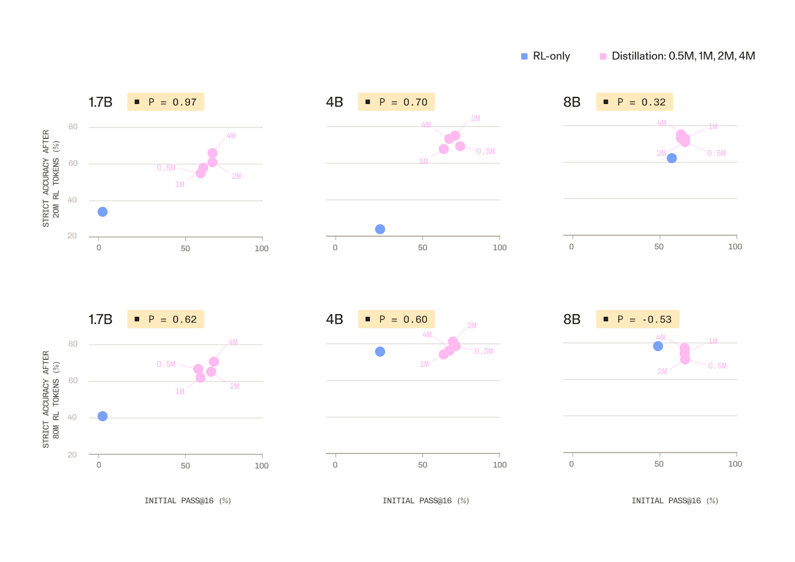
figurea7 — Figure 13
Initial pass@16 against strict accuracy after 20M RL response tokens (top) and 80M tokens (bottom). Each student size has five points: RL-only and SFT doses of 0.5M, 1M, 2M, and 4M teacher-response tokens. ρ is Spearman’s rank correlation across those five conditions.

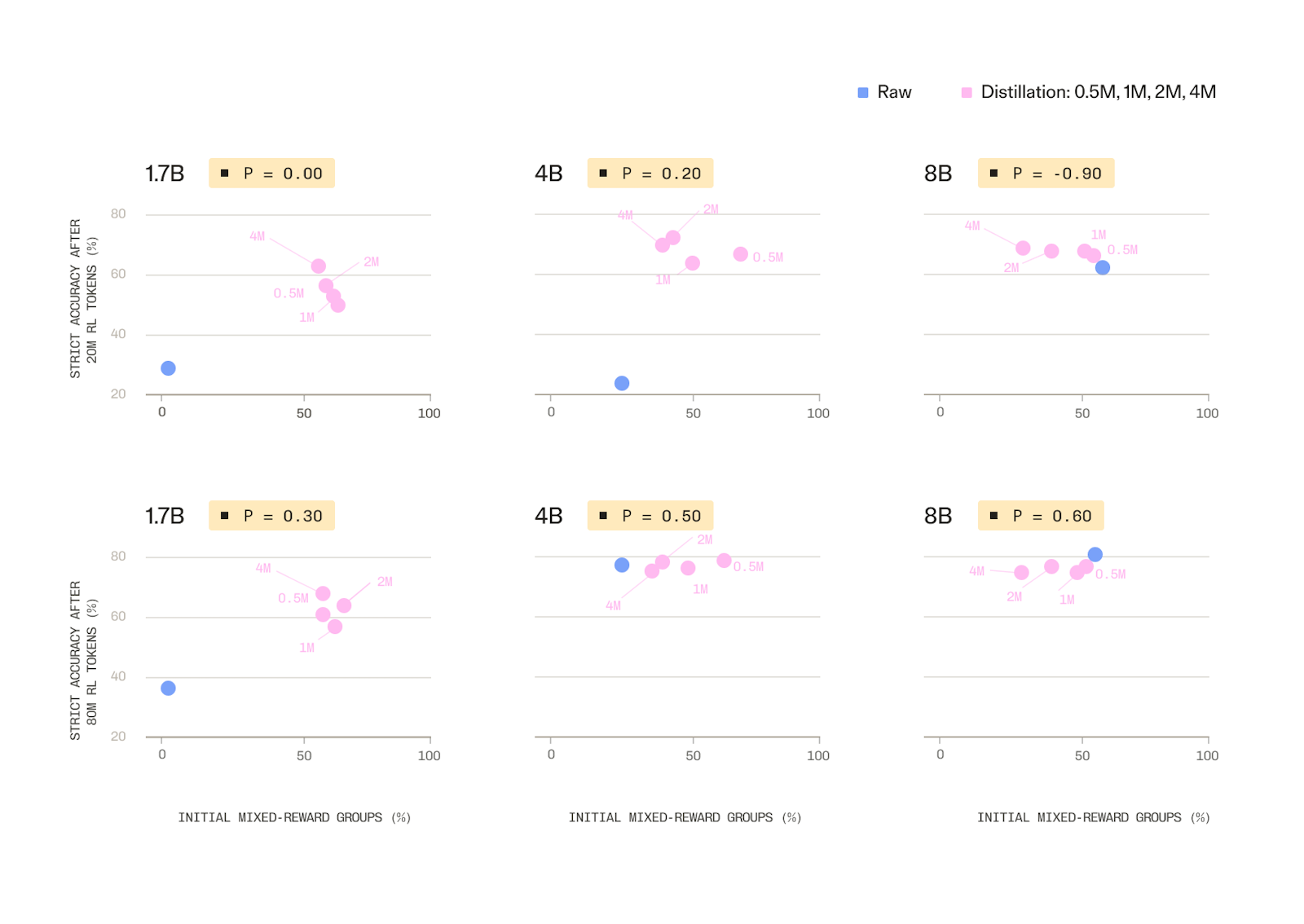
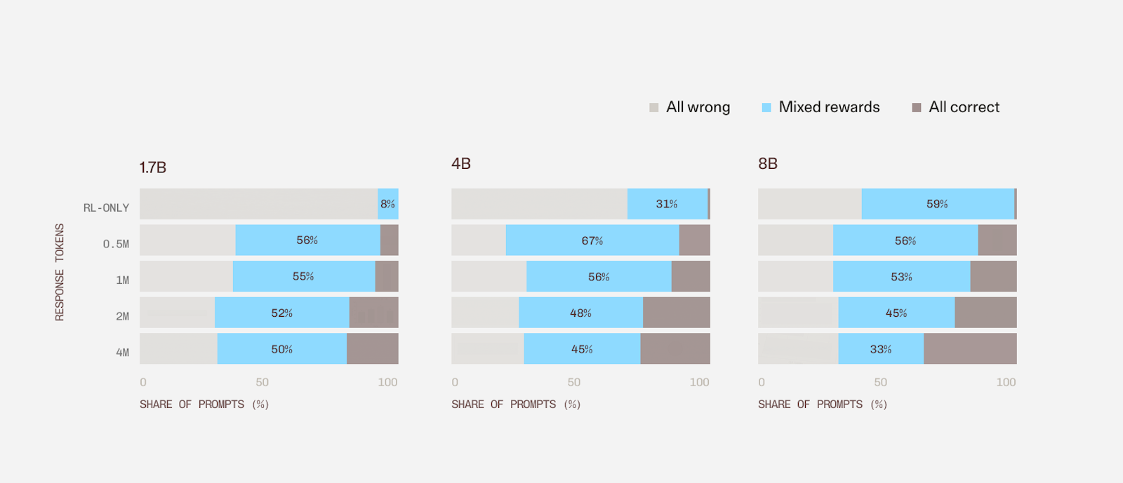
figurea9 — Figure 15
Composition of 16-response groups before RL for the RL-only starting policy and four SFT amounts at each student size. Each bar gives the share of prompts whose sampled responses are all unrewarded, mixed, or all rewarded.

For a prompt with $n=16$ sampled responses and $c$ correct responses, the finite-sample pass@k estimator is:

\widehat{\mathrm{pass@}k}=1-\frac{\binom{n-c}{k}}{\binom{n}{k}}.

The numerator is zero when fewer than $k$ failures are available. We compute this per prompt and average equally across tasks. All-wrong, mixed, and all-correct fractions are counted directly from the same groups. These records use the standard-task training sampler, temperature 1.0 with top-k disabled, rather than the main evaluation decoder.